A summer of boats, bears and bugs

Lawrence Eagle, University of Leeds

Last year my summer was filled with adventures: June was occupied by a hiking expedition across a remote part of Swedish Lapland, whilst late July and most of August were filled with my first visit to new PhD field sites in South East Alaska. Although I had never visited the region before my supervisors had and there is a wealth of academic and lay literature about the region, its geomorphology and ecology. So before I had even boarded a plane, let alone the ferry or small landing craft to be used throughout the field season, I believed I knew what was to come.

Figure 1. Three young brown bears fishing for pink salmon in a stream mouth. Bears posed a major logistical challenge as sites were often inaccessible as a result of their presence.

However, accessing sites through thick willow and alder scrub, where the only passable route is along the tracks forged by brown bears, is hard. Tracking the thalweg of a waist deep, boulder laden stream whilst recording on a cumbersome GPS unit… and watching for the aforementioned bears is harder. That’s before you mention the accidental dips into the freezing waters of the bay; the pieces of kit that are lost downstream after slipping on slimy boulders in the middle of a stream; failing to buy suitably water resistant electronic scales and dodging icebergs as we cruised up the bay towards its remaining glaciers. Nonetheless my first taste of the wilds of Alaska and of fieldwork in such a changeable environment were addictive.

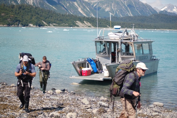
Figure 2. Field team disembarking the research vessel the Capelin. Credit Dr Lee Brown

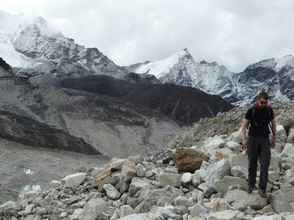
My research catchments are located in Glacier Bay National Park, which was first established as a National Monument in 1925 under pressure from a number of eminent conservationist including John Muir and William Cooper. Now the national park is part of a UNESCO world heritage site and a United Nations biosphere reserve. The region has experienced rapid deglaciation since the 1700s, exposing a bay 150km long and 20km wide. Research here has focussed on glacial retreat, changing environmental conditions and the succession of ecosystems from bare ground through to coniferous forests. This succession of communities from bare ground to forests results in a diverse range of both terrestrial and aquatic ecosystems within the bay. As you move up the bay (and streams get younger) streams display a decrease in habitat complexity and a shift from slow flowing habitat types (such as pools and glide) to fast flowing habitat types (such as rapids and riffles).

Figure 3. Map of Glacier Bay with principal research catchments marked in white. Age of streams in brackets.

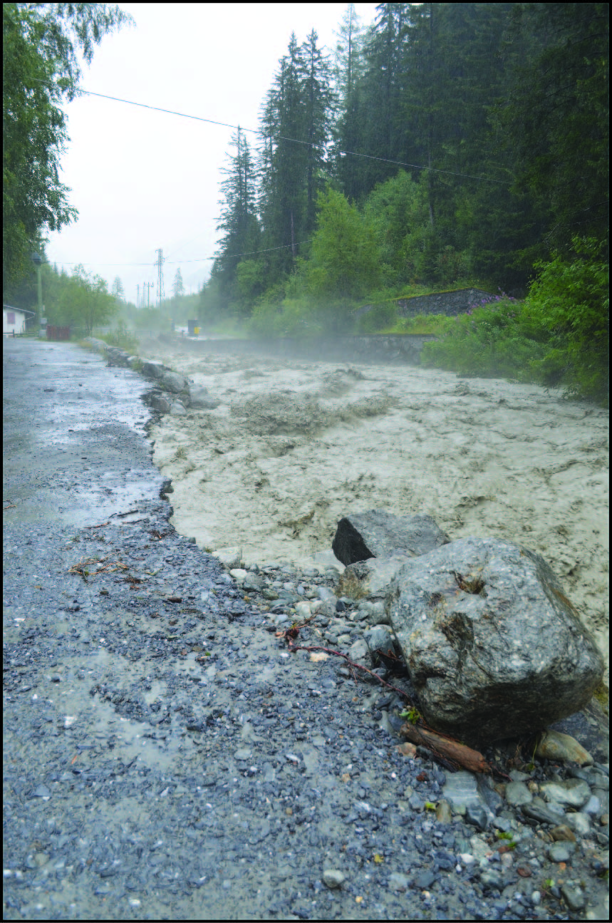
The summer of 2014 saw atypical, persistent, heavy rainfall across much of South East Alaska, driving sustained and repeated flood events in Glacier Bay throughout June, July and August. These floods form the primary focus of my PhD, which is interested in how stream ecosystems respond to extreme flooding and the role habitat availability and complexity play in conferring resistance to, and resilience following floods.

To understand how an ecosystem responds to a disturbance event it is important to understand how habitat availability and complexity, before and after the event, may drive ecological processes and community change. As such my project has two main aims: to quantify habitat change and availability associated with the floods and to quantify how the ecosystem responds over a number of years.

Figure 4. Waterfall and plunge pool holding over 1000 pink salmon at Wolf Point Creek.

There is a long history of stream research in Glacier Bay, focussed on ecological and geomorphological succession. As such I have access to a broad range of secondary datasets collected, in the main by my supervisors, over the last 40 years. My task was to identify the most relevant pieces in these datasets and then collect data to allow for comparisons of pre and post flood conditions. Understanding how habitat availability affects response in a diverse range of species with drastically different life history traits (think fast moving juvenile Coho salmon versus tiny midge larvae clinging to a rock) requires an equally diverse approach.

Consequently, my habitat mapping work has three main strands; mapping channel geomorphic units (CGUs) along 1km long reaches; repeating regularly collected cross sections at study sites and sampling sediments in an attempt to understand variation in microhabitat availability for aquatic invertebrates. These activities were pursued at all of my study sites in an attempt to elucidate the role of both meso and microhabitat in ecological response to disturbance.

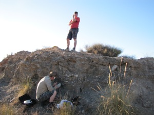
Figure 5. Dr Megan Klaar resurveying longstanding cross sections. Credit Dr Lee Brown

Mapping CGUs is a slow process which occupied the majority of time at each field site. The process requires an individual to identify CGUs based on a hierarchical system, combining visual and physical characteristics of the river channel and flow at any given point, and then to walk the thalweg of the CGU with a mapping grade GPS. The process is then repeated for all CGUs along the study stretch to produce a CGU map of the river. This presents a number of challenges. Walking the thalweg through deep pools is often dangerous, and at times impossible due to their depth, whilst the thalweg of rapids can have such a high flow rate it is almost impossible to walk with or against it the flow. Secondly, consistently allocating CGUs to the correct category across sites with numerous physical differences and ensuring this is repeatable from one year to the next was challenging. Reaches were mapped from the tidal extent of the stream in an upstream direction until at least 1km had been mapped or to any structures (high falls) impassable to salmonid fish (a group of particular interest to the study).

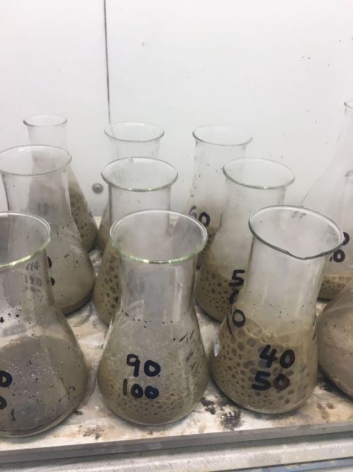
Due to the time consumed mapping CGU’s there was less time than anticipated to focus on other fieldwork goals. The field team successfully rerecorded cross sections which will add to long standing datasets. Additionally some microhabitat data collection was possible, however only a limited number of sediment measurements were taken at each site, instead of a comprehensive analysis originally proposed. This will now become a major focus of future field campaigns.

In addition to this habitat data, aquatic invertebrate larvae, fish and algal samples and data were collected to allow us to map how ecosystems and communities of these organisms respond to the floods through time. These samples represent another core topic of my PhD.

Figure 6. Collecting aquatic invertebrate samples. Lawrence Eagle (Author, far right), Prof Sandy Milner (Centre) and Captain Todd Bruno (napping, far left, after safely guiding us up bay in his vessel the Capelin). Credit Dr Lee Brown

Now I am beginning the arduous task of processing geomorphological data and biotic samples (this requires me to identify thousands of individual bugs – before dissecting them and identifying their stomach contents!) in advance of a proposed second field season through the summer of 2017.

Figure 7. Channel geomorphic unit map of Wolf Point Creek.

The field season was supported by the BSG, water@Leeds and the Staffordshire Educational Endowment fund and I offer my thanks to each of these organisations for their continued support.

 

A summer expedition – Indian Himalayas – Anne Stefaniak

I recently returned from a 3-week expedition to the Indian Himalayas with the British Exploring Society. Having previously lead on expeditions with BES as a science leader to Arctic Norway and Svalbard, I decided it was time to venture further afield – to the Himalayas.

British Exploring expeditions aim to develop Young Explorers through challenging situations with a good dose of science thrown in! While in the Himalayas we discussed and looked at a whole range of scientific disciplines including botany, lake sediments, geology, meteorology, geomorphology and by no means least, glaciology! Each science leader had their own area of expertise and designed suitable projects for the explorers to contribute to including identifying various plants and soils and looking at pollination methods. One project incorporated glacial geomorphology and glaciology, looking at the way glaciers had shaped the landscape we were camping in. This involved mapping large moraines systems using Google Earth imagery prior to the expedition which was then ground truthed with data collected in the field during the expedition.

Geomorphological mapping of the expedition region in Ladakh using Google Earth imagery (completed by expedition participants prior to the expedition).

Of course when on expedition, or fieldwork for that matter, nothing ever goes exactly to plan; especially when dealing with altitude and young people. It took us 4 days to slowly make our way to basecamp at Pensi La due to the steady acclimatisation period. We travelled from Leh located at 3505 m up to 4400 m. Even arriving in Leh, the effects of altitude could be felt but with some rest and taking it easy for a day or so we were able to head towards our basecamp. Once at basecamp we spent a few days training and gaining skills such as ice axe arrests and walking on difficult terrain. After the training phase we managed to get onto the Drang Drung glacier and camped in the valley. The Drang Drung glacier is heavily debris-covered on the right hand side and enabled us to have a look at some of the impacts of debris on a glacier system. For many it was their first experience of being on a glacier and proved to be the highlight of the trip. In addition to exploring the glacier, we explored the ridge behind basecamp and managed to exceed 5000 m of altitude.

Ice skills training including ice axe arrests and students taking a break viewing the Drang Drung glacier.

It was a great expedition with the YE’s being able to get involved in all sorts of science projects, camp life and even our own expedition Olympics! We left the 5 week expeditioners at basecamp in Pensi La and made our journey back to Leh via Kargil.

Walking back to basecamp after a long day hiking. View of the Leh monastery which overlooks Leh.

To find out more about the expedition see the BES Science Journal detailing the science projects which will be available online later this year.

Anne Stefaniak is a PhD student at Nottingham Trent University and the BSG Postgraduate Deputy Chair. The expedition was undertaken with the British Exploring Society.

How we spent our summer…

It has been a busy summer for all members of the postgraduate forum whether that be on fieldwork, completing laboratory work or writing papers. The focus of this blog is to find out what each member of the forum has got up to this summer so we can demonstrate the diversity of a geomorphological PhD!

Scott Watson, University of Leeds

‘One of my main activities this summer was a five week field trip to the Khumbu Glacier in Nepal. This was the second of three trips to gather field data for my PhD and I also used the opportunity to climb a 6000 m peak on a day off. Aside from that, I’ve been writing the second paper towards my PhD, which is investigating ice cliff dynamics in the Everest region using fine-resolution satellite imagery. I’ve also been easing my way back into trail running following a lengthy injury (acquired during the first field trip), and preparing for my final field trip in September.’

Francesca Falcini, University of York

‘It’s been a relatively quiet summer for me in terms of fieldwork, but I did attend the QRA field meeting to Skye in May. Lots of glacial landforms and rock slope failures to see, which make for an amazing landscape that lives up to the hype. Perhaps the most exciting part of the trip was being in the presence of not just one but both Benn and Evans, who arguably wrote the glaciology bible.  I also enjoyed a week in Ireland helping fellow BSG postgrad forum rep Lauren with her fieldwork. In between those trips I’ve been in the office working on my upgrade documents, method development and planning papers.’

Rachel Hurley, University of Manchester

‘It has been a relatively uneventful summer for me with a solid block of labs, barring one week in the Cretan mountains. I’m working to finish off all of my analytical work before the new term so that I can get my head down in my writing up year. I have also been putting together the first publication from my PhD  – it will be exciting to see my work out in print!’

Danielle Alderson, University of Manchester

‘After the wonderful summer that I had last year visiting Florida followed by an undergraduate field trip to India, I have unfortunately been experiencing solely the climes of Manchester this year! As I approach my submission pending year I have largely been glued to my chair in front of my desk analysing data for my third and fourth papers as part of my PhD. I generally seem to have two computers open at all times in addition to something on Netflix to keep me sane! It finally feels like everything may begin to come together at some point soon which is certainly a very exciting feeling and one that every PhD student seeks. I have had a busy September, firstly attending the Plymouth AGM (particularly the conference dinner in the National Marine Aquarium!) followed by an undergraduate field trip to Keswick and finally a week away in Turkey!’

Lauren Knight, University of Portsmouth
‘It’s been a very busy and exciting summer, full of fieldwork. In May I was back in the Wicklow Mountains, Ireland, for a second (very sunny) field season. I also attended the QRA Skye Field Meeting, where the geomorphology was amazing. In July I helped a colleague with fieldwork atHardangerjøkulen in Norway. We camped on the southern side of the ice cap and collected a lot of useful data in some challenging conditions. Finally, in August I returned to Wicklow for my third and final field season. Despite horrendous weather I managed to finish all the required geomorphological mapping and sedimentology. I even managed to continue triathlon training with several local runs and evening swims in a nearby lough. Now I’m back in the office, starting on analysis, which feels very strange after busy and active summer!’

Anne Stefaniak, Nottingham Trent University

‘This summer I spent 3 weeks in the Indian Himalayas in Ladakh with a group of young explorers on expedition with the British exploring society. The aim of the expedition was to take the young explorers to a new environment and look at a range or scientific and adventure projects. As well as going on the Drang Drung glacier and climbing our way up to over 5000 m of altitude, we also had a go at learning a variety of scientific techniques. The projects ranged from geology, meteorology, lake studies, geomorphology and not least glaciology! The work from the expedition will be presented on a few different posters at the BSG conference this September.’

Daniel Sperl, University of Cologne

‘When Danielle asked me about my PhD life summer activities, I first thought: “Daniel, what did you do during summer and what should I write about?” My summer was very diverse: (1) I stayed away from Cologne for one month at the catholic university at Louvain-la-Neuve to prepare samples and discuss my work with my co-supervisor. (2) After I returned, I helped pack our “collection of stones” (more than 3 t of rocks), due to the reason that our department is moving into a new building. (3) I attended a summer school in Germany on “Dates and Rates of Change in Quaternary”. It was a great week, meeting friends that I made during the Windsor Workshop last year. We had a great time together and are planning a future trip to the Highlands of Scotland. (4) Finally most of my time was spent writing papers during a rainy summer here in Cologne, as is displayed in the picture!’

Owen King, University of Leeds

‘Like Scott, the biggest focus of my summer so far has been preparing for and carrying out a second field season in Nepal. We were back in the Khumbu valley this May to repeat surveys we carried out last October/November, and I’m currently working through the processing of this second huge batch of data. Some preliminary results look really exciting though, and the rate at which the Khumbu glacier is changing and losing ice is really alarming. Sadly that’s my fieldwork completed now, but the next couple of months should be really interesting writing the fruits of my labour up into a second paper towards my PhD.’

We hope fellow postgraduate members of the society also had wonderful summers! Please get in contact if you would like to tell us about them, or if you have anything you would like to raise with the postgraduate section of the society!

Danielle Alderson (danielle.alderson@manchester.ac.uk)

Twitter- @BSG_Postgrads

Facebook- BSG Postgraduates

 

Fieldwork report: Khumbu Glacier, 2015

By Scott Watson

Back in October, Owen King and I travelled to the Khumbu Glacier in Eastern Nepal, accompanied by two of our supervisors Duncan Quincey and Ann Rowan. The aim was to collect field data on how the glacier is thinning year-on-year, and to validate and improve our satellite remote sensing observations that have been the focus of our PhDs prior to fieldwork.

Location of our field site in the central Himalaya

The Khumbu Glacier is the highest glacier in the world and every year a small section of it becomes the home to Mount Everest Basecamp. Travel to the glacier involved a seven day walk from the nearest airstrip at the village of Lukla, which included two acclimatisation days to cover our ascent from 2,800 m to ~5,000 m. The highest elevation we reached (excluding a brisk jaunt up the small trekking peak Kala Patthar) was ~5,300 m at an unusually quiet Everest Basecamp, which was deserted following the recent earthquake.

Our campsite (left) and the lower debris-covered area of the Khumbu Glacier (below)

Everest region background

It’s widely known that debris-covered Himalayan Glaciers in this region are losing ice mass year on year, although the presence of a thick layer of sand and rocky debris delays their response to climate change. The glaciers are currently out of equilibrium with climate, and will continue to thin irrespective of any contemporary slowdown in climatic warming. The debris cover, which is generally thickest at the terminus of the glaciers and becoming thinner at higher elevations, changes the spatial distribution of melt. Generally speaking, highest melt rates occur where the debris is thin or absent, whereas thick debris insulates the ice beneath.

Supraglacial ponds (i.e. existing on the surface) and ice cliffs are widespread on the low-gradient, debris-covered areas of the glaciers. Ice cliffs can range from several to tens of metres high, and ‘ponds’ can be over 100 m in diameter. Although data are limited, it is thought that ice cliffs and ponds contribute highly to overall melt at a glacier scale. At ice cliffs, bare ice is melted by incoming solar radiation, and ponds are similarly warmed and transmit this thermal energy to the ice below, or through conduits draining into the glacier.

The area of surface water ponding is increasing on the Khumbu Glacier and individual ponds are coalescing, which are likely to form a large glacial lake in coming decades.

Field data

The debris-covered area of the Khumbu Glacier is ~10 km long and the lower ~5 km is stagnant, whereas flow exceeds 60 m a^-1 in the ice fall. Our work was predominantly in the lower 6 km where ponds are coalescing and large ice cliffs were present.

The high-altitude rugged topography, hazardous access, and unstable behaviour of the debris-covered glaciers means that field data area limited and hard-earned. Crevasses are minimal on the lower Khumbu Glacier but ice cliffs and topographic highs are constantly changing as the ice melts beneath. The hummocky topography was unstable and would often slump, making it hard to cover any nominal distance. Each hummock was essentially a rocky, ankle-twisting version of the Gladiators Travelator. Our Nepali guides were invaluable in this environment for route finding and helping carry our field equipment. A fine-resolution satellite image base map on a GPS device also made locating the cliffs and ponds considerably easier.

Ice cliffs: structure-from-motion and multi-view stereo (SfM–MVS)

A photographic survey tailored to the requirements of the SfM-MVS workflow was conducted around each ice cliff selected for study, which basically requires photographing the environment from as many different locations as possible (i.e. 1- 2 hours clambering around the Khumbu Travelator). Specialist software (e.g. Agisoft Photoscan) is able to match the images and create a 3d point cloud representing the ice cliff and surrounding environment. Visible ground control points were distributed around each cliff and georeferenced with a dGPS before the photographic survey so the model could be scaled and georeferenced.

A preliminary example, which can be navigated in 3D is available at: http://www.rockyglaciers.co.uk/explore/ice_cliffs.html

Example of a 3D ice cliff model

Pond surveys

The ponds forming on the surface of the glacier can broadly be split into two classes: those with active meltwater inflows (e.g. from adjacent ice cliffs), and those that are hydrologically isolated from any melting ice and thought to be relatively stable through time. My monitoring strategy involved deploying thermistor strings in a range of ponds to measure their thermal regime. These temperature loggers were deployed using an inflatable dinghy (christened HMS Khumbu), which was kindly borrowed from a fellow PhD student also working in Nepal. Most ponds were frozen at their surface by the end of the campaign, so access though ~10 cm of ice was required for logger retrieval (an ice screw/ ice axe combo worked well).

During our next field campaign, I plan to collect distributed depth measurements across a number of ponds to derive bathymetry, and hence determine the water storage volume of the ponds.

Deploying temperature loggers in a supraglacial pond

__________________________________________________________________________________

Scott Watson is a PhD student at the University of Leeds and a BSG Postgraduate Committee member. Scott’s fieldwork in 2015 was supported by a University Research Scholarship, the Royal Geographical Society, the British Society for Geomorphology, and water@leeds.

http://www.rockyglaciers.co.uk/

________

Planning and undertaking fieldwork

By Lauren Knight, Portsmouth University.

Giving August 2015 was a very wet month in Ireland, particularly in the Wicklow Mountains. It was also the month that I headed into the area for the first field season of my PhD. This was my first ever field season, before August I had never undertaken independent fieldwork for more than a week and I learnt a lot of valuable lessons along the way. I thought I would use this blog to share a few of these.

The Wicklow Mountains lie south of Dublin in the Republic of Ireland. The area is largely protected by a National Park and covers more than 200 km². It is an area steeped in history; home to a 6^th century monastic settlement in Glendalough, the site of the 1580 Irish rebellion battle of Glenmalur and the source of water for the Guinness Brewery in Dublin. It is also an outstandingly beautiful region, (but then I’m biased) and there are also abundant glacial features.

 

Location and relief of the Wicklow Mountains, Ireland (52°53’N-53°15’N; 06°11’W- 06°36’W)

In brief, my PhD seeks to use a combination of geomorphological mapping, sedimentology and dating techniques to establish the dynamics and timings of Late Devensian glaciation within the Wicklow Mountains. Although it is largely accepted that the area hosted an independent ice cap at the Last Glacial Maximum (LGM), little work has focused upon the shift to localised mountain glaciation during the Last Glacial-Interglacial Transition (LGIT). Even less is known about the extent and nature of glaciation during the Younger Dryas (YD), although the area contains the type-site for the YD in Ireland (Lough Nahanagan). My PhD research hopes to address some of these gaps.

Mapping amongst the ferns (in some places these were over head height, not so good feature identification)

One of the exposures that will be revisited in 2016, when sedimentology becomes the field focus

Fieldwork is a huge part of data collection for the project and will be undertaken over three fieldwork campaigns. As I’ve already mentioned, the first happened in August. That month was perhaps one of the most intense and mentally demanding experiences I’ve had (so far). It was challenging and hard work throughout, but I enjoyed it immensely! I was finally in the field looking at sites that I’d stared at on Google Earth and in Arc Map for months. It was so satisfying to have actually reached this critical stage of my PhD, after months of reading and planning. Plus the evidence that I was finding was exciting!

Here are a few lessons I learnt along the way, which may help you if you’re planning fieldwork for the first time:
1) Check your field kit thoroughly beforehand

If you think some of your field kit looks a bit worse for wear, seriously consider the benefits of replacing it before that extended field season. My walking boots were pretty old, but faithful and very comfortable. I knew that they needed replacing soon but felt that I didn’t have time to find the perfect new pair, let alone break them in before fieldwork. However, four days into the season the sole of my left boot peeled neatly off. This was very inconvenient. Fortunately, a short journey to an outdoor retailer rectified this little problem… but what if I had been at a remote field site? If I had been in the Arctic or Himalayas… my neat new boot solution would not have been an option. My oversight could have seriously jeopardised the success of the fieldwork, compromising my ability to cover large distances safely and quickly. Duct tape and superglue can’t really compete with a waterproof and fully soled boot. (For the record, I love my new boots we bonded spectacularly – no blisters!)

The beginning of the end of the faithful boot – it got a lot worst.

 

2) Be ambitious, but be realistic and adaptable.

My field schedule was packed. I had a master plan of all the key sites that I had to visit and I spent a lot of time trying to work out the best way to maximise the time in the field. Car access and parking for each site was planned, the most direct walk-in routes were figured out and even multi-valley days were scheduled to cover as much ground as possible. The one thing I didn’t plan was the weather. Persistent low cloud, along with days and days of heavy rain meant that it just wasn’t possible to cover the distance I’d planned in saturated, boggy terrain. It also meant that I didn’t manage to get into some sites at all. A few hanging valleys remained heavy in cloud every time I visited. Yet, I had recognised that plans need to be adaptable –before fieldwork I’d prepared for a number of contingency days. These were low levels days that I should be able to cover rain or shine. In hindsight I can see that I was overambitious with my original plan, but it did mean that I had prepared to cover a large area in detail. This also meant that when the weather made some sites unfeasible, I had a range of back up sites – not just my handful of contingency days. It was only really towards the end of the field season, after a month of poor weather that I started to struggle with site selection.

When planning fieldwork I think its useful to try to consider what might go wrong and prepare for that. I suppose we have to try to expect the unexpected (easier said than done I know) – but always try to have a back up plan. It doesn’t need to be a complicated, but try to pre-empt what might jeopardise your plans. What could you do if a piece of field equipment gets damaged? Can you make a temporary ‘fix’ for it? Do you have spare base maps for when yours get destroyed by rain? What will you do if you can’t get access to a site?
If you try to think about potential problems, specific to your fieldwork, before they happen you can be better prepared to deal with the issues in the field. We all put a lot of time and effort into our field plans; it is incredibly frustrating when things don’t go to plan. So do what you can to try to avoid that field disaster.

Hiding behind a rock to try to get some shelter to map

Still enthusiastic about moraines… for now (we left when the thunder and lightning started, that day ended a little early)

 

3) Lone field working – is it for you?

Sometimes it can be difficult to find field assistants, especially if you’re in the field for an extended period of time. You may find yourself considering some time in the field on your own. I had a week of lone working and that was enough time for me to establish that I really like having some company in the field. It is worth taking the time for find out whether lone working is for you before deciding upon a prolonged period of solo fieldwork. I would also advise checking your University’s lone working policy – it might be that you’re not permitted to venture out alone; in this case the decision has been made for you!

In my opinion a helpful field assistant is invaluable. If they’re knowledgeable about the subject area then you can have discussions in the field (vocalising what you think you’re seeing/is happening can really help clarify your initial thoughts). Even if they’re not familiar with the topic, a good field assistant can get stuck in to make your data collection even more successful – an extra pair of hands is very practical and helpful. Plus, when you’re in the field for a prolonged period even the most passionate and dedicated researchers can find their enthusiasm waning after a while. By the final week of fieldwork, when even my waterproofs were struggling with the rain, my field assistant helped keep the energy levels high (we laughed a lot) and we had a very productive week (we mapped a lot). It was almost certainly a far more constructive than I think it would’ve been if it had been my forth solo (and soggy) week in Ireland.

Even swarms of bugs can’t stop a good field assistant being an excellent scale

 

Neither will rain dampen an enthusiastic take on ‘get in the photo for scale’

 
Plus it’s nice to have someone to share your lunch with after you crawl through peat.

 Said peat crawling incident… a last resort. We sank quite quickly otherwise.

Overall, I had a fantastic time in Ireland and learnt a lot very quickly on my first field season and I hope that sharing some of these will help some of you plan your first field season. In brief, we all know how important kit is to get us through tough ground conditions. A kit oversight meant I wasted half a day and added unnecessary hassle early on in the trip. Don’t make foolish kit mistakes like me! Check your kit thoroughly. Also have back up plans (multiple)! Careful preparation meant that even when things didn’t go to plan, I could still get out there and maximise my time. So try to be organised for when things go wrong (something will!). Similarly, I now realise that fieldwork can be incredibly lonely and that I’m a creature of conversation. In fact talking through my initial thoughts with someone made me work much more decisively and efficiently. So for me, having company in the field improves not only the volume (and quality) of data collected, but also the experience getting that data. I think that’s really important, for all of us! As PhD students we are enthusiastic about our work but we should also try to have a good field experience. Think carefully what type of person you are in that respect before heading out solo!
My final (extra) tip is that sometimes you’ve just got to walk away for the day. Fieldwork is intense and it is okay to take a small break when things get tough. The time can still be useful and productive. Perhaps use that time to write up your field notes, or rethink your plan for the next week. Also, use that time to eat some well-deserved cake.

Fieldwork is tough. Cake is good. We’ve earned it.

All that’s left to say now is – good luck with your fieldwork!

Lauren Knight, Portsmouth University.

 

 

Apps in the Field: PDF Maps

Rupert Bainbridge, Northumbria University

Back in May I was lucky enough to get to go on some fieldwork to New Zealand, travelling to some pretty remote locations. Having done some similar fieldwork in the past one thing I didn’t want to do was cart around a laptop and charger with me as the journey out is quite long and the weight limit can be a bit restrictive if you have a lot of fieldkit. To this end I decided to take a tablet with me instead, granted it still needed a charger but it’s much lighter and less bulky to carry around.

I decided to have a look into how useful a tablet might be actually in the field rather than just in down time and came across an app called PDF Maps, many of you reading may have come across it and used it before. Personally I thought it was a great addition to the fieldwork arsenal and has some useful functions for the field researcher.

Loading Maps

OK, so initially you obviously need to have an internet connection to load up maps, but one of the apps best features is that once you’re set up it can be used completely offline! The maps are stored on the device, not run from the internet.

When I’m talking about maps with this app, it’s really any piece of georeferenced material; satellite/aerial imagery, geology maps, topo maps, geomorph maps etc., so long as the files have been prepared correctly they’ll all work. There are a couple of methods for putting maps onto your tablet for the app to use.

• Download them using the in-app store. There are a number of different types of map available, in the store, I usually just click the ‘find maps’ option at the top and navigate to where I’m going to look at the range of things available in my destination. Luckily for me most of the topo maps in NZ are available for free and they’re listed in the app, so simply download and they’re ready to go. Alternatively there may be a small fee for downloading the maps, you can click on the available maps and see what price certain maps are.
• Prepare the maps yourself in ArcGIS. OK, so the maps you want may not be available through the app or they might be too expensive. Good news is that you can quickly and easily make them using ArcGIS, I haven’t tested this on QGIS mind you. I had a number of aerial images that I wanted to export and use in the field, some of them were already annotated and some blank, either is fine as the final product will just be a georeferenced PDF, so you can have some features already highlighted for when you’re in the field.

I’m not going to go through the whole process but there’s a great video for making the maps for the app (https://vimeo.com/79337719), they talk about the I-Pad in the video but I used the same process on an Android OS and it works a charm.

Figure 1: Overview of the PDF Maps app store showing available maps for the South Island, NZ and the information for the Springfield tile. No price is shown here as this map is freely available

Finally once the maps are exported you need to transfer them to the tablet and load them into PDF Maps. I used Dropbox as an easy solution to this as there is an option within the app to directly import from a Dropbox app. PDF Maps lets you make folders and subfolders for organising anything you’re loading in (Figure 2) and will tell you if the georeferencing on the map isn’t working.

Figure 2: (Left) List of folders created by the user and (Right) the contents of the 1:50000 map folder showing the downloaded maps from the map store.

Using PDF Maps in the field

 So once everything is loaded in and you’re finally at your fieldsite there are a couple of handy functions that can be used (Figure 3):

• Locate function: Like most phones these days, tablets usually have some sort of GPS function. A quick press of the locate button and you’ll have a pretty decent location for yourself in the field, I found this particularly useful for roughly locating myself on aerial imagery and topo maps when the scale of the maps weren’t quite as small as I would have liked.

• Placemarks: A placemarks function lets you put ‘pins’ on your imagery. The app just places the pin in the centre of the screen (using the bullseye symbol) so it can either be used in conjunction with the locate function and be placed on your location or you can pan around the map and place them where you like. Opening each placemark then lets you edit the description and name to whatever suits you. Photos can also be added to the placemarks, either directly from the device or at a later date from the device or other file sharing apps like Dropbox.

As a quick note, I haven’t tested the absolute accuracy of the positions given in the app against a handheld GPS or a dGPS. However when I was using this app I did try to get it to locate me in known locations and it was actually surprisingly accurate for the most part (around 5-10m) and even found me in some very remote locations when my handheld GPS wasn’t able to locate me. I suppose this matters depending upon how you plan to use the app.

• Measure Distance or Area: This does exactly what it says on the tin. Using your maps the app can estimate distance and areas (2D). It’s a bit clunky, but using the centre point you can create lines and polygons which then give a readout. I used this mostly for estimating some distances in the field to calculate walking times from place to place but it could of course be used for much smaller scale jobs.

• Jump to adjacent maps: You can also use the arrow buttons on the screen to jump to a menu which will show you nearby maps to the one you’re currently viewing. It’s a simple case of selecting the map you want to see. My NZ maps were labelled sequentially which helped when jumping from map to map.

Figure 3: Screenshot from an individual map in PDF Maps showing the various functions available. The example used is a NZ topo map however the view is the same for any map you have imported to the app.

All in all I found it a very easy app to navigate both in terms of loading maps and using it in the field to locate myself and log placemarks and descriptions of features. The maps were easy to prepare and load and the function buttons are really quite intuitive. Ultimately I found it quite useful for being able to take lots of imagery and maps into the field without carrying bundles of paper around and trying to keep everything dry.

For the fieldwork I did also buy a waterproof cover (Proporta Beachbuoy) for the tablet which worked very well in some pretty wet conditions!

Working with the tablet in the field (whilst neither of the pictures show rain I can assure you it happened…)

An Overview of Observations and Impacts of the 26th August 2014 Val Veny floods

By Rupert Bainbridge, Northumbria University

So I was recently in the European Alps helping out on some fieldwork for a colleague, Mark Allan. Whilst we were there to look at landslides onto glaciers the weather quite often had other plans! On the 26^th August 2014 in Val Veny, Italy we had some heavy, but as I’m told for the summer of 2014 not unusually heavy rainfall, which caused extensive damage to infrastructure and rapid channel change. So, unable to reach our landslide fieldsites, fuelled on delicious European pastries and with a flooding river we were unable to resist the urge to document some of what happened that day. Below is a brief overview of some observations and impacts from the flooding.

Val Veny is the main trunk valley for ~7 alpine glaciers. However the Brenva and Miage glaciers are the only ones that currently flow into the valley bottom. The river is heavily managed using gabions, boulder riprap and engineered channelisation. Figure 1 shows a number of sites visited during and after the 26^th September flood to monitor changes during and look at the impacts after the event.

Figure 1: Satellite image of Val Veny showing the major glaciers and the locations of the sites discussed below. Click the picture fore a higher resolution version!

Site 1: Campsite access road, Pertud

The first site we visited, conveniently, was the access road and bridge to our campsite (Site 1). At this site the river is channelised by permanent walls along its southern bank above and below the bridge; boulder riprap is used to protect the bank upstream of the bridge whilst permanent wall structures are used to protect the banks downstream (Figure 2A).  Unfortunately we missed the flood peak, but caught it on the waning stage.

The bridge in Figure 2 was restricting flow causing localised overbank flooding. Some minor infrastructure damage occurred here with debris on the roads, some large woody debris within the bridge structure and localised scour around boulder riprap which had eroded sections of bank, damaging the road (Figure 3). Interestingly ice inclusions were found in some of the debris washed up onto the bank (Figure 2B), which indicated to us at the time a possible glacial source for some of the flood water.

Figure 2: (A) Main road and Perthud access bridge showing the channelised river in waning stage. The red dashed line shows debris indicating the peak flood height; (B) Example of ice inclusion in flood debris.

Figure 3: Localised scour on the campsite access road. Boulder riprap upstream of the road cut show evidence of scour suggesting this may have been the initiation mechanism for the road erosion.

Site 2: Miage Glacier

Access to the Miage Glacier was possible on the 27^th September, the day after the floods. During this visit that there were a number of small freshly drained supraglacial lakes along the eastern margin of the glacier which are thought to have contributed to the flood waters. However on this trip we did miss the big smoking gun! A colleague Tom Shaw ventured to the Miage glacier in late September to collect some monitoring equipment and aside from some of the equipment disappearing in the flood, the glacial Lake Miage had drained as well (Figure 4). Combined with other possible supra-glacial lake drainages there could have been a significant glacial contribution to the August 26^th flood.  Some anecdotal evidence suggests that there may also have been lake drainages on the Freyney Glacier.

Figure 4: The basin of the former Lake Miage. The red line approximates the previous lake surface. (Photo credit: Thomas Shaw)

Site 3: Freney track wash-out

                One of the more impressive impacts of this relatively small flood was the Freney farm track wash-out. Having been running on this track in blissful sunshine just the day before it was impressive to see very little evidence of the road having existed in the first place! A number of avulsion channels were present through the forested area where the road had been, one following the general path of the road. The channel headcut seen in Figure 5 appears to have continued migrating upstream between our visits on the 26^th (A) and 27^th (B).

Figure 5: Channel avulsion on the Freney farm track. (A) During the August 26^th flood, note the channel headcut which is not present the following day; (B) August 27^th return visit, the dashed line approximates the line of the road and the circle indicated the same boulder in each photo.

Fresh boulder and debris run-ups behind trees in Figure 6 highlight the competence of the flow to transport large material through over a large area (not just in channelised flows) and the extensive impact at this site.

Figure 6: Large scale boulder deposition through the forested area near Freney

Site 4: Road and bridge wash-out, Brenva Glacier/Mont Blanc Tunnel

                One of the last sites we visited on the 27^th (due to road closures) was near the bottom of the Brenva Glacier. There were extensive ice-cored moraine complexes being undercut by the floodwaters (Figure 7). As a result of this, large quantities of superficial sediment was collapsing into the flood flows and being reworked downstream.

Figure 7: Superficial sediment collapse into flood waters

                A little further downstream one of the access roads to the Mont Blanc Tunnel crosses the river. The bridge surface itself had survived but much of the surrounding area had been severely eroded. Head-cuts on either side of the bridge surface had cut it off completely, whilst it is clearly evident from the boulders over the bridge surface that flows had been much higher and transporting large material (Figure 8).

Figure 8: Bridge and road damage on one of the Mont Blanc access roads. The red dashed line indicates the old road surface. Black dashed lines indicate erosion scars, some of the lower scars to the right of the bridge may be abandoned head-cuts. Black arrows indicate the active river channels, each of which is an active channel head-cut.

Hopefully this has been an interesting overview of the flash flooding we saw on August 26^th 2014, they were certainly impressive on the day! There are some videos taken by Mark on the new BSG Postgraduate YouTube page:

https://www.youtube.com/channel/UC8hpjsVUcUL0DrXoEowu6lA/videos

79 North vs 80 South

By Kate Reid, Northumbria University

My mum always says that wherever I go, the sun goes down when I leave. That is not to say that her world is darkened when I leave my hometown in Scotland, but more that when I leave my field sites, the midnight sun begins to lurk beneath the horizon, if only for a few hours or so. My interest in all things icy started, rather appropriately, in Iceland during a geography class trip when I stood on my first ever glacier and immediately caught the glaciology bug. Having spent last boreal summer in Svalbard (79 degrees North) and the recent austral summer in Antarctica (80 degrees South) I can tell you that I still haven’t managed to shake off my first love!

  Summer at Pyramiden, 79 degrees North and Independence Hills, 80 degrees South

However, the two regions couldn’t be much further apart, both geographically and metaphorically speaking. Grassy squares, derelict buildings and two Russian workers greeted me upon arrival at 79 degrees north in the northern archipelago of Svalbard. In contrast an immaculate silent, white landscape with a smattering of distant mountains was all that I could see when our British Antarctic twin otter plane circled around our desired camp site, trying to find a suitable landing spot in amongst the steep sided sastrugi. The impeccably pristine environment of our field site in Antarctica could hardly have been more of a contrast to that of the abandoned town of Pyramiden that I visited 6 months previously, with its imported grass, broken windows and rusting iron. Was this the fate Antarctica narrowly missed out on? Saved by the Antarctic treaty, which permits only peaceful endeavors and scientific observations to be carried out there?

Pyramiden: an abandoned Russian coal mining town in Svalbard

Putting political matters and debatable land use issues aside and moving onto my more selfish needs, it was fantastic to swap my long and tedious night-time patrols of camp armed with a flare gun and rifle in Svalbard for a peaceful night’s sleep in Antarctica.

 Fashion styles in Svalbard and Antarctica differed somewhat!

However, sleeping was not only a night time treat in Antarctica – it gradually became a daytime routine as ever more frequently the 40 knot katabatic winds and extremely poor visibility kept us from carrying out radar traverses and geological investigations of Patriot Hills, in Horseshoe Valley, West Antarctica. To begin with the rest days were welcome, but as they dragged on and worries of how to collect the remaining data crept in, I started longing for the warmer days in the north. My mind wandered back to Svalbard where life flourished – with arctic terns and puffins aplenty, along with lush vegetation and countless crevasses and meltwater streams to jump over or inject with Rhodamine dye.

 Meltwater stream investigations in the warmer climate of Svalbard

So do I have a preference?  Well, not really. Despite the obvious differences in landscape and swapping the odd encounter with a bear, with numerous penguins at Rothera base station, I feel equally at home in both places and can’t wait to go back!

Adélie Penguins at British Antarctic Survey’s Rothera base station, Adelaide Island, Antarctica

The Himalayas and Me

By Morgan Gibson, Aberystwyth University

‘Oh me, I’m a glacial geologist, sort of, who studies the effect of climate change on Himalayan glaciers’ – the response I give when I am, frequently it seems, asked what I do. I always ruffle my feathers remembering how lucky I am when I get to say that. Then the moment is shattered when the question all PhD students dread is asked: ‘So what do you want to do once you’ve finished?’

 

My name is Morgan and I am the newest member of the BSG Postgraduate forum. Currently I am in my first year of my PhD at Aberystwyth University, trying to reconstruct Himalayan glaciers through the Quaternary, and then having a go at projecting these change into the future (basically lots of fancy computer programs I don’t quite understand yet…), with a focus on trying to work out what role rock debris on glacier surfaces play in the whole thing. The bonus of this is 10 weeks fieldwork around Everest base camp this year, quite a perk !!

 

So why the Himalayas? Well it has been a bit of an obsession of mine since I was young – big scary mountains, lots of ice, cool looking temples, lots of silly people trying to summit said scary mountains. It was pretty similar to my expectations when I visited Nepal in my gap year, and I fell in love with the place. On my return I headed to Edinburgh for my undergraduate degree, getting involved in the Royal Scottish Geographical Society, the Uni. Expedition Society and Brathay Exploration Group, the latter of which let me lead expeditions to Norway to explore glaciers. All of this put me in the mood for some adventure, and got me a bit obsessed with glaciers. So, when I moved to Aberystwyth, it was time to combine my sense of adventure and the Himalayas. And here I am today, looking forward to my time as part of the BSG Postgraduate forum!

 

Morgan Gibson

Twitter

Research page

Post Field Season Blog

By Martin Geach

Tabernas Basin: Tectonics Vs. Climate

A big hello to all new & existing BSG Postgraduate members, I hope the research is going well and post-Christmas life is just grand. I have recently returned from my third field season in the Tabernas basin in SE Spain and thought I would take a little time to enlighten you all on my recent exploits!

Research Focus: Briefly summarised my research is focused on the Quaternary evolution of the Tabernas basin in SE Spain. As such the study aims to assess (qualify/quantify) the significance of external drivers (tectonics, climate) in the evolution of the basin landscape spanning back to the latest Pliocene.

Tabernas Basin: The basin itself forms just one of a series of Neogene intramontane sedimentary basins of the Almería region in SE Spain (Fig. 1). Broadly speaking the Almeria region is characterised by a series of major extant ranges (sierras) and intramontane sedimentary basins, that have formed due to north-south compressional tectonic regimes throughout the Mid-Tertiary (Sanz de Galdeano & Vera, 1992). The emergence of the region via tectonic convergence resulted in a change from marine to continental conditions and, during the Quaternary, the switch to basin inversion and rapid incision of drainages (Harvey et al., 2003).

Figure 1 – Digital Elevation extract for the Almerίa region, SE Spain. Date sourced from: Instituto Geográfico Nacional, Spain

Across the basin the vast range of geomorphological styles, as attributed to the effects of Quaternary tectonics and climatic change, has created a landscape of spectacular diversity and beauty that has even been the base for numerous movies in the recent past (e.g. A Fistful of Dollars, Indiana Jones and the Last Crusade, etc.). In the east, the basin is characterised by a series of climatically controlled coalescent alluvial fan sequences with a typically featureless topography. In contrast, the west of the basin demonstrates the significance of on-going tectonics with some 250m of post-inversion incision, forming a landscape dominated by deeply entrenched bedrock fluvial systems and badlands (Fig. 2).

Figure 2 – Major geomorphological features of the Tabernas Basin. A: Morphological map of major Quaternary landscape units, B: Travertine Curtain at Las Salinas, C: El Cautivo Badlands

Fieldwork: So how do you assess the significance of tectonics and climate in a sedimentary basin? – Well in the case of the Tabernas basin we focus on extensive preserved landscape surfaces and isolated fluvial terraces that record both stages of tectonic uplift (creation of accommodation space/down cutting of drainages) and periods of climatic dominance. My task is to make sense of these major cut/fill style landscape levels in order to assess their interactions over a range of spatial and temporal scales across the basin (Fig.3). Ultimately unravelling the spatial complexity of the landscape surfaces requires a good degree of time in the field, with the resultant mapping of surface levels after intensive reconnaissance. Field mapping is made slightly easier with what I term- ‘Martin’s Magical Field Kit’ (might have been alone in a basin for slightly to long!). In my field kit I have all basic tools for logging/locating sections, but in addition I carry the Trimble TruPulse360- a fantastic laser sighting device that enables remote measurements of horizontal & vertical distance, slope distances, azimuth and inclination. Typically the TruPulse has a range of approx. 300m for sighting and works in most conditions, however readings can be limited by humidity or in the case of Dartmoor blanket fog! Recently I have also added the Trimble Juno unit to my ‘magical field kit’- this windows based field unit running ArcPad10 software can be utilised in the field to assess topographic levels, directly map features or take digitally referenced field photographs.

Figure 3- Quaternary landscape levels in Rambla Buho. A: Field photograph of landscape surfaces, B: Comparison image formatted in ArcGlobe10 utilising 5m Ortho-corrected digital imagery and elevation data, soruced from Instituto Geográfico Nacional, Spain

Assessing the temporal nature of sequences across the basin is deeply rooted in the spatial relationships and interactions of units. In simplified terms I am looking to formalise relative stratigraphic levels across the basin and understand how these levels relate to each other both in terms of elevation and sedimentology. This relative stratigraphy is, hopefully – touching lots of wood, going to be supplemented by absolute dates obtained from Optically Stimulated Luminescence (OSL) dating (Fig.4). Finally the outcomes from this research will enable the qualification and quantification of extrinsic drivers upon long-term landscape evolution within the Tabernas basin (easy as that – I wish!!).

Well that is all from me for now, if you have any questions/ feedback with regard to my research or the equipment I use in the field please contact me via email or on twitter.
Take care and happy new year!!
Martin Geach

Figure 4- Field gamma-spectrometry within OSL sampling location in upper surface of terrace remnant. Note supervisor for scale- not too sure about the slight militant stance.

References:

Harvey, A. M., Foster, G., Hannam, J. & Mather, A. E. (2003) ‘The Tabernas alluvial fan and lake system, southeast Spain: applications of mineral magnetic and pedogenic iron oxide analyses towards clarifying the Quaternary sediment sequences’. Geomorphology, 50 pp 151-171.

Sanz de Galdeano, C. & Vera, J. A. (1992) ‘Stratigraphic record and palaeogeographic context of the Neogene basins in the Betic Cordillera, Spain’. Basin Research, 4 pp 21-36.